Why can a respectable Brier score still hide a specific failure?

Brier score is one number averaged across all probability bins. A trader who is well calibrated in the middle of the probability range and badly miscalibrated at the tails can post the same Brier score as a trader who is mediocre everywhere. The two profiles need different fixes. The shape of the calibration curve, not the headline score, tells you which one you are.

How do you build a calibration curve from your prediction market trades?

Bin every logged probability you put on a trade (typically 10 bins from 0-10% to 90-100%). For each bin, compute the average probability you stated and the actual fraction of those trades that resolved YES. Plot stated probability on the x-axis and actual frequency on the y-axis. Perfect calibration is the 45-degree diagonal. Deviations above or below the line are the diagnosis.

What does the shape of your calibration curve tell you?

An S-shape (overconfident at high probabilities, underconfident at low ones) is the classic overconfidence pattern documented in Lichtenstein, Fischhoff and Phillips (1982). A reverse-S means underconfidence at the tails. A curve consistently above the diagonal means systematic underestimation; below means overestimation. The shape tells you which probability range needs recalibrating, which the headline Brier score cannot.

Calibration curve, plainly. · Reading between the Markets

Predictive Labs @Predictive_Labs

‘A 0.10 Brier hides a 90% disaster.’ Brier is one number. Two traders with the same 0.10 score can have completely different problem profiles, and they need completely different fixes. A calibration curve plots stated probability against actual frequency, binned across all the trades you logged. Perfect calibration is the 45-degree diagonal. Above the line means you are underestimating; below means you are overestimating. The shape, not the average distance from the diagonal, is the diagnosis. The classic overconfidence pattern (Lichtenstein, Fischhoff and Phillips 1982) is an S-curve: well-calibrated in the middle, overconfident at high probabilities and underconfident at low ones. Common in retail PM trading. The fix is to compress your tail probabilities toward the centre, not to shift everything. A respectable Brier with a bad curve shape will keep losing money in a specific way. The curve says exactly where.

9:30 AM · 4 May 2026 0 Views

In plain English

A trader logs 200 probabilities on Polymarket and Kalshi over six months and computes their Brier score: 0.10. Respectable. Better than the platform aggregate, in the same neighbourhood as published superforecaster benchmarks. The trader concludes their probability calls are sound and continues sizing trades on the same logic.

Six more months later, the book is down. The Brier score has not moved much. The thing that changed was that a particular kind of bet (high-conviction calls priced in the 80s and 90s) has been resolving against the trader more often than the stated probabilities implied. Brier did not see it because the bins where it happened were a small fraction of the total. The calibration curve would have shown it the first time it was looked at.

Why a respectable Brier score can hide a specific failure

Brier is one number averaged across every prediction the trader logged. It rewards getting close to the actual outcome, on average, and it does not care which probability bin the closeness came from.

Two traders can post identical Brier scores while making very different mistakes. Trader A is well calibrated everywhere, evenly close to the diagonal across the probability range. Trader B is excellent in the middle (40% to 60%) and dramatically off at the extremes, with calls priced at 90% resolving more like 75% and calls priced at 10% resolving more like 25%. Averaged across a portfolio that mostly lives in the middle of the price distribution, the two profiles produce nearly the same headline Brier. They demand opposite responses. Trader A should look at sizing and selection. Trader B should compress their tail probabilities and re-examine the conviction logic that produces 90s and 10s.

Brier is the right scoring rule for forecasting (proper, decomposable into reliability and resolution components). It is the wrong tool for diagnosis. A single average cannot tell the trader where in the probability range the model breaks. The calibration curve does, with no extra inputs.

How to build a calibration curve from your trades

Three columns of data are enough: the probability the trader stated before the trade, the eventual outcome (1 for YES resolved, 0 for NO resolved), and the date. Polymarket and Kalshi store the market price the trade hit, not the probability the trader believed. The trader has to log their own number before each trade for this to work.

The procedure:

1. Bin the stated probabilities. 10 bins of 10 percentage points each is the textbook default (0-10%, 10-20%, ..., 90-100%). Wider bins (5 bins of 20pp) work for smaller samples; narrower bins need 500+ observations to be stable.

2. For each bin, compute two numbers. The average probability the trader stated within that bin (x-coordinate). The actual fraction of trades in that bin that resolved YES (y-coordinate).

3. Plot the bins. X-axis is stated probability, Y-axis is actual frequency, both 0 to 1. The diagonal y = x is perfect calibration. Each bin is one point.

4. Check sample size per bin. A bin with 5 observations is noise. A bin with 50+ is informative. Display the count next to each point so the eye does not over-read sparse bins.

The curve is the line connecting the bin points. Where it sits relative to the diagonal is the diagnosis. The shape is what matters.

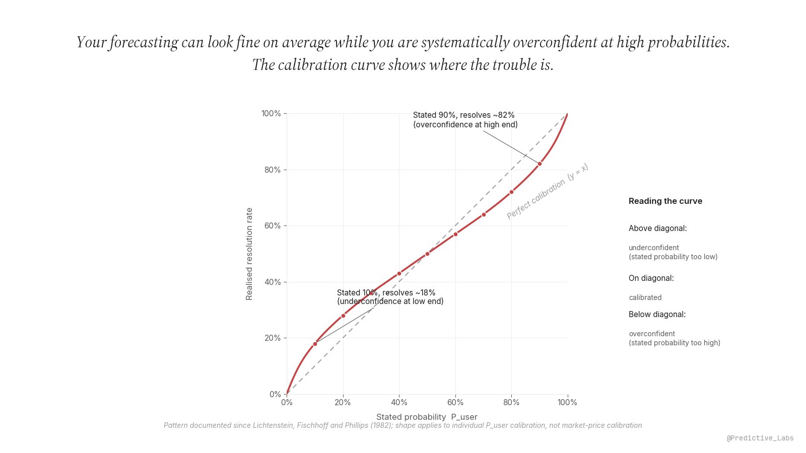
Reading the curve at three example bins

Stated bin Actual frequency Diagnosis 10-20% (avg 15%) → 22% = underconfident 40-60% (avg 50%) → 49% = on the line 80-90% (avg 85%) → 72% = overconfident

Same trader, three bins, three different diagnoses. The middle of the range is fine. The high-probability bin is where the money is leaking, and a tail-only recalibration is the fix.

What the shape of your curve tells you

Four canonical shapes carry distinct diagnoses.

S-curve (the classic overconfidence pattern). Above the diagonal at low probabilities, below it at high ones, crossing through the middle. This is the dominant pattern in the early calibration literature (Lichtenstein, Fischhoff and Phillips 1982 review of the state of the art to 1980, included in the Kahneman, Slovic and Tversky Heuristics and Biases volume). It says the trader compresses uncertainty too aggressively at the extremes. The fix is to pull tail probabilities back toward the centre: when the conviction-driven model wants to say 92%, write 84%; when it wants to say 7%, write 14%. Mid-range probabilities should be left alone.

Reverse S-curve. Below the diagonal at low probabilities, above it at high ones. Less common but seen in traders who systematically discount their own conviction (under-extreming). The fix is the opposite: trust the tail calls, since they are more right than the stated probability suggests.

Curve consistently above the diagonal. Actual frequency exceeds stated probability everywhere. The trader is systematically underestimating. Often a sign of overcautious framing or implicit hedging in the probability log itself.

Curve consistently below the diagonal. Actual frequency is lower than stated probability everywhere. Systematic overestimation. Common in traders who anchor on their own conviction without enough deference to the base rate.

The market-side counterpart to the S-curve is the favourite-longshot bias documented in the Kalshi data (Whelan 2026): low-priced contracts win less often than their prices imply, and high-priced contracts win slightly more often. A trader whose own curve mirrors that pattern is replicating the market’s mistake rather than profiting from it.

How this lives in nijinn

The Performance Audit Surface in nijinn builds the calibration curve directly from the trader’s logged probabilities and the resolved outcomes of their Polymarket and Kalshi trades. The curve is rendered with sample-size weighting on each bin, the diagonal is overlaid, and the deviation pattern is classified against the four canonical shapes. The headline Brier is shown alongside (linked to the Brier Score companion entry), so the trader can see both the average and the shape on the same panel.

The metric pairs naturally with the directional sizing logic from Quarter Kelly: a trader whose curve overestimates at the high end is, by definition, sizing too aggressively on their highest-conviction calls, since those are the ones the Kelly fraction loads up on. Recalibrating the tail of the curve fixes the sizing problem without changing the rule.

A respectable Brier with a bad shape is a slow leak. The curve shows the trader where the leak is and what to fix.