Why is more hedge to compensate for low correlation backwards?

Standard minimum-variance theory (Johnson 1960) sets the optimal hedge notional at the correlation between the two legs multiplied by the volatility ratio multiplied by the exposure. As correlation drops, the optimal notional drops with it. Adding more contract notional at low correlation increases the variance of the hedged book, often beyond the variance of leaving the exposure unhedged.

What is the minimum-variance hedge ratio formula?

The minimum-variance hedge ratio is h* = correlation multiplied by (volatility of exposure / volatility of contract). Multiply by the exposure size to get the dollar notional of contract to take. When the two legs have similar volatility, this simplifies to correlation multiplied by exposure.

Why do binary prediction-market payoffs sharpen the hedging problem?

A Polymarket or Kalshi contract pays $1 or $0 with no partial credit for a partial event. That makes contract returns structurally lumpy and adds a discreteness to contract variance that continuous futures do not have. The minimum-variance formula still applies, but the variance estimates have to capture the binary jump rather than treating the contract as a smooth proxy.

How do you size a prediction-market hedge in practice?

Estimate the correlation between the contract resolution outcome and the underlying exposure, estimate the volatility of each leg, compute h* = correlation times (volatility of exposure over volatility of contract) times exposure, and place that dollar notional of contract. Re-estimate as new information arrives. Hedge size scales down with correlation, not up.

Hedge ratio, plainly. · Reading between the Markets

Predictive Labs @Predictive_Labs

‘Adding hedge can add risk.’ A treasurer with $500K of inflation-sensitive exposure considers $1M of Kalshi CPI contracts, reasoning that imperfect correlation calls for more notional to compensate. The math says the opposite. At 0.50 correlation with similar volatility on both legs, $1M of contract produces a hedged book roughly 3 times more volatile than the unhedged exposure. Contract noise dominates everything else. Standard hedging theory (Johnson 1960, every CFA and FRM curriculum) sets optimal notional at correlation × volatility-ratio × exposure. Where the two legs carry similar volatility, that simplifies to correlation × exposure. $500K at 0.85 correlation calls for roughly $425K of contract. At 0.70, $350K. At 0.50, $250K. Lower correlation means smaller hedge. Binary PM payoffs sharpen this. No partial credit for a partial event, so contract variance is structurally lumpy. The discipline is to scale notional down with correlation. A treasury hedged to its headline exposure when the underlying correlation is low is the most common way to be over-protected on paper and over-exposed in practice.

9:30 AM · 3 May 2026 0 Views

In plain English

A treasurer at a mid-cap distributor sees $500,000 of headline exposure to a CPI surprise next month. They consider Kalshi’s CPI contract as a hedge. The contract correlates with their actual cost-pressure exposure at maybe 0.50, since the headline CPI prints differently from the basket of inputs the firm actually buys. The instinct: buy more notional than the exposure to compensate for the imperfect correlation. $1M of contract, maybe $1.5M.

The instinct is wrong by a factor large enough to flip the sign of the trade. Standard hedging theory says the optimal contract size shrinks with correlation, not grows. This entry is about the formula every textbook treats as foundational and that retail hedging on Polymarket and Kalshi routinely inverts.

Why ‘more hedge to compensate for low correlation’ is backwards

The intuition behind over-hedging at low correlation is that imperfect coverage demands extra size. The math says the opposite, because contract notional brings its own volatility into the book.

A hedged position has two sources of variance. The original exposure carries its own. The contract carries its own. The two interact through their correlation. When correlation is high (the contract closely tracks the exposure), the two variances mostly cancel and the hedged book is much less volatile than either leg alone. When correlation is low, the cancellation is partial. Adding more contract notional past the optimal size does not get you closer to a flat book; it adds standalone contract variance that the partial cancellation cannot absorb.

The result: at a correlation of 0.50 with similar volatility on both legs, taking $1M of contract against $500K of exposure produces a hedged book whose variance is roughly 3 times the variance of leaving the exposure unhedged. The treasurer reaching for more notional has not bought protection; they have bought a directional bet on the contract whose payoff happens to partly correlate with their underlying.

The minimum-variance hedge ratio, plainly

The standard formula (Johnson 1960, restated in Stein 1961, Ederington 1979, every CFA and FRM curriculum since) sets the hedge ratio that minimises the variance of the hedged book at:

h^* = ρ × (σ_S / σ_F)

where ρ is the correlation between the change in the exposure and the change in the contract, σ_S is the volatility of the exposure leg, and σ_F is the volatility of the contract leg. The optimal dollar notional of contract to take is h^* multiplied by the exposure size.

When the two legs carry similar volatility (a reasonable approximation in many treasury hedging cases), σ_S divided by σ_F is roughly 1 and the formula collapses to the simple form:

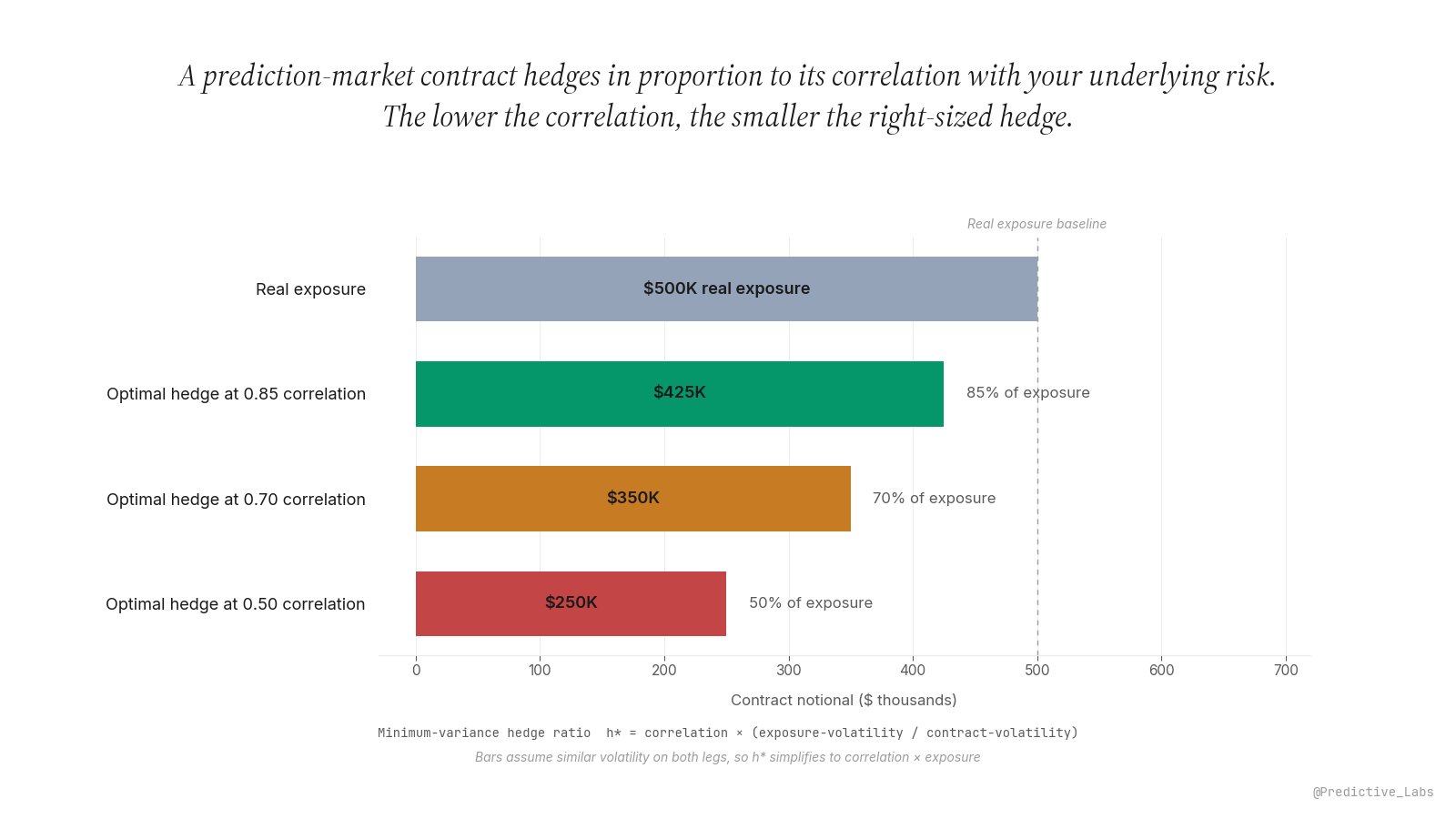
Optimal contract notional ≈ ρ × Exposure

which is the version the diagram above visualises. Notional scales linearly with correlation. There is no scenario under standard assumptions where lower correlation calls for more contract.

Optimal hedge size on $500K exposure (similar volatility)

Correlation Optimal notional % of exposure ρ = 0.85 → $425,000 = 85% ρ = 0.70 → $350,000 = 70% ρ = 0.50 → $250,000 = 50%

The optimal contract notional is the correlation times the exposure when volatilities match. The variance reduction the hedge actually delivers is ρ-squared (Ederington 1979): 0.72 at 0.85 correlation, 0.49 at 0.70, 0.25 at 0.50. The remaining variance is basis risk.

Why binary PM payoffs sharpen the problem

The minimum-variance derivation was developed for futures contracts, which are continuous claims with smooth payoff curves. Polymarket and Kalshi contracts are not. They pay $1 if the event happens and $0 if it does not. There is no partial credit for a partial event.

Binary payoffs add structural lumpiness to contract variance. A continuous-futures hedge tracks small spot moves with small contract moves. A prediction-market hedge gives the user nothing during the contract life (price moves on Polymarket and Kalshi are still continuous, but the realisation of payoff is binary at expiry) and then a 100-cent jump at resolution. The total contract variance over the holding period is dominated by that resolution jump, especially for contracts that resolve far from 50/50 where the day-to-day price changes are small relative to the eventual settlement.

The formula still applies. What changes is how the contract volatility σ_F has to be estimated. Treating the contract as a smooth proxy and using only intraday price moves understates its true variance. The correct estimate captures both the path volatility before resolution and the resolution jump itself, weighted by the probability of each outcome. Sloppy estimates here are how a binary contract that looks like a clean hedge in normal-day variance ends up adding more risk than it removes when resolution day arrives.

How to size the hedge in practice

Five steps, in order, every time:

1. Define the exposure precisely. What is the dollar amount at risk, what time period does it cover, and what specific event drives the loss? ‘Inflation exposure’ is too vague. ‘$500K of cost increase if April CPI prints above 0.3% month-over-month’ is the version the formula works on.

2. Estimate the correlation. Either from historical co-movement of the underlying with similar past contracts, or from a structural argument about how the contract’s resolution maps to the firm’s exposure. A treasurer hedging a basket-specific CPI exposure with a headline CPI contract is starting at correlations well below 1.

3. Estimate the volatilities of both legs. Use the holding period that matches the hedge horizon. For PM contracts, factor in the resolution-jump component, not just the path volatility.

4. Compute the optimal notional. h^* times exposure. Cross-check by computing the residual variance the hedge leaves; if the post-hedge variance is higher than the pre-hedge variance, the formula has been mis-specified.

5. Re-estimate. Correlations drift, volatilities drift, the resolution date approaches. The optimal notional from a month ago is rarely the optimal notional today. A static hedge against a moving correlation is not a hedge.

How this lives in nijinn

The Real-World Hedging Surface in nijinn computes the minimum-variance optimal notional for any exposure-to-contract pair. The user inputs the exposure size, picks the candidate Polymarket or Kalshi contract, and nijinn estimates correlation from the contract’s historical resolution behaviour against the user-defined exposure proxy, estimates volatilities including the resolution-jump component, and surfaces the optimal contract notional plus the expected variance reduction (ρ-squared). Adjusting the correlation assumption updates the optimal size live.

The metric pairs naturally with the basis-risk and Meta-Market mapping disciplines on the arbitrage side: a PM contract whose resolution wording does not exactly match the exposure is a contract whose true correlation is lower than the headline implies. Cross-link to P_user versus market price on the directional side, since hedge-driven trades and edge-driven trades follow different sizing logic and should not be confused.

A hedge sized to the exposure is the wrong hedge. A hedge sized to the correlation is the trade.